Getting Started with NumPy: Arrays, Installation and Why NumPy Is Fast

If you have worked through our Python Fundamentals series, you already know how to store numbers in a list and loop over them. That works well for a handful of values. It starts to hurt when you have a million sensor readings, a spreadsheet of exam marks or the pixels of an image. NumPy is the library Python developers reach for at that point, and almost every data and AI tool you will meet later (pandas, scikit-learn, PyTorch, OpenCV) is built on top of it.

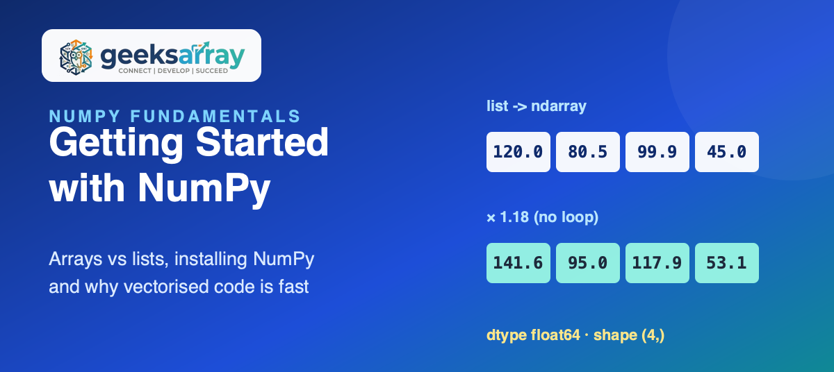
This is the first part of our NumPy Fundamentals series. By the end of it you will have NumPy installed, understand what an array is and how it differs from a list, and see for yourself why NumPy code is both shorter and much faster.

What NumPy actually is

NumPy (Numerical Python) gives you one central object, the ndarray: an N-dimensional array of values that all share the same type. Because every element has the same type and the values sit next to each other in memory, NumPy can hand whole calculations to fast, compiled C code instead of running a Python loop element by element.

That single design choice explains most of what you will learn in this series:

• Same type everywhere means an array of numbers is just numbers, with no per-element Python objects to look after.
• Contiguous memory means operations stream through the data quickly.
• Vectorised operations mean you write prices * 1.18 instead of a loop, and NumPy applies it to every element.

Installing NumPy

NumPy is a third-party package, so install it with pip. It is a good habit to do that inside a virtual environment, exactly as we did in the Python series, so each project keeps its own versions:

python -m venv .venv
source .venv/bin/activate        # Windows: .venv\Scripts\activate
pip install numpy

Everyone imports it under the short name np. It is such a strong convention that you will see np. in every tutorial, answer and codebase:

import numpy as np
print("NumPy version:", np.__version__)

All examples in this series were run on NumPy 2.3.4.

Your first array

The simplest way to make an array is to pass a list to np.array:

prices = [120.0, 80.5, 99.9, 45.0]
arr = np.array(prices)
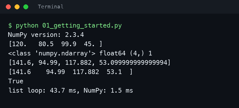
print(arr)
print(type(arr), arr.dtype, arr.shape, arr.ndim)

[120.   80.5  99.9  45. ]
<class 'numpy.ndarray'> float64 (4,) 1

Four attributes describe every array, and you will check them constantly:

• dtype is the type shared by every element. Here it is float64, a 64-bit floating-point number.
• shape is the size along each dimension. (4,) means one dimension holding four values.
• ndim is the number of dimensions: 1 for a row of values, 2 for a table, 3 for something like a colour image.
• size (not printed here) is the total number of elements.

Notice how NumPy prints the array: no commas, and the numbers lined up. That is your quick visual clue that you are looking at an array, not a list.

The same job, list vs array

Suppose every price needs 18% GST added. With a list you write a loop, or a list comprehension from the collections post:

print([p * 1.18 for p in prices])
print(arr * 1.18)

[141.6, 94.99, 117.882, 53.099999999999994]
[141.6    94.99  117.882  53.1  ]

The NumPy version has no loop at all. arr * 1.18 multiplies every element, and the result is a new array. (The 53.099999999999994 versus 53.1 is the same floating-point value; NumPy simply prints it rounded.)

This style is called vectorisation: you describe what should happen to the whole array and NumPy does the looping in compiled code. It is the single most important idea in NumPy, and we spend all of Part 4 on it.

Why NumPy is fast

Let us measure it. We will sum the squares of the numbers from 0 to 999,999, first with a plain Python generator over a list and then with NumPy:

import time

n = 1_000_000
data = list(range(n))
big = np.arange(n)

t = time.perf_counter(); total = sum(x * x for x in data); t_list = time.perf_counter() - t
t = time.perf_counter(); total_np = int((big * big).sum()); t_np = time.perf_counter() - t
print(total == total_np)
print(f"list loop: {t_list * 1000:.1f} ms, NumPy: {t_np * 1000:.1f} ms")

True
list loop: 35.5 ms, NumPy: 4.4 ms

Both give the same answer, and NumPy is roughly eight times faster on this machine. The exact numbers will differ on yours, but the gap only widens as the data grows. For heavier work, such as matrix maths, the difference is often a hundred times or more.

When to use a list and when to use an array

NumPy does not replace lists. Use each where it fits:

• Use a list for a small, mixed collection: names, a few settings, items you append to one at a time.
• Use an array when you have many numbers of the same kind and want to calculate with all of them: marks, prices, measurements, coordinates, pixels.

Arrays are also fixed in size. Appending to an array creates a whole new array, so the usual pattern is to collect values in a list first and convert once with np.array.

NumPy in the real world: an image is an array

Once you know arrays, you start seeing them everywhere. A colour photo, for example, is simply a 3D array: height × width × 3 colour channels (red, green, blue), each value a number from 0 to 255. Here is a tiny 4×6 "image", left half red and right half blue:

img = np.zeros((4, 6, 3), dtype=np.uint8)
img[:, :3] = [255, 0, 0]     # left three columns: red
img[:, 3:] = [0, 0, 255]     # right three columns: blue
print(img.shape, img.dtype, img.nbytes)
print(img[0, 0], img[0, 5])

(4, 6, 3) uint8 72
[255   0   0] [  0   0 255]

uint8 is an unsigned 8-bit integer, exactly 0 to 255, so each pixel channel takes one byte and the whole image takes 4 × 6 × 3 = 72 bytes. A real 1920×1080 photo is the same idea with about 6 million values. Libraries such as Pillow and OpenCV hand you images as NumPy arrays, so brightening a photo is a single expression, and cropping it is the slicing you will learn in Part 3.

The same is true across data and AI work:

• pandas stores each column of a table as a NumPy array.
• scikit-learn takes training data as a 2D array: one row per example, one column per feature.
• Audio is a 1D array of samples, and video is a 4D array of frames.
• Deep-learning libraries such as PyTorch use tensors that convert to and from NumPy arrays with one call.

That is why NumPy is worth learning properly before any of those tools: the shapes, slicing and broadcasting you learn here are the same ideas you will use in all of them.

Practice exercises

Try these before reading the answers.

1. Make an array from the temperatures [31.5, 29.0, 33.2, 35.8, 30.1] and print its dtype, shape and size.
2. The thermometer reads 2.5 degrees too high. Correct every value without a loop.
3. Predict, then check: what do np.array([1, 2]) + np.array([3, 4]) and [1, 2] + [3, 4] each give?

temps = np.array([31.5, 29.0, 33.2, 35.8, 30.1])
print(temps.dtype, temps.shape, temps.size)
print(temps - 2.5)
print(np.array([1, 2]) + np.array([3, 4]), [1, 2] + [3, 4])

float64 (5,) 5
[29.  26.5 30.7 33.3 27.6]
[4 6] [1, 2, 3, 4]

The last line is the key lesson of this part: the same + adds arrays element by element but joins lists.

Common mistakes

• Expecting + to join arrays. With lists, [1, 2] + [3, 4] gives [1, 2, 3, 4]. With arrays it adds element by element and gives [4, 6]. Use np.concatenate to join, which we cover in Part 5.
• Looping over an array element by element. It works, but you lose the speed. Look for the vectorised form first.
• Mixing types in one array. np.array([1, "2", 3]) silently turns everything into strings. Keep arrays to one kind of data.

Wrapping up

You have installed NumPy, created your first array, read its dtype, shape and ndim, and seen vectorisation beat a Python loop. Next, in Creating NumPy Arrays, we look at all the ways to build arrays without typing every value: ranges, evenly spaced values, zeros, ones, random numbers and choosing the right dtype.